Recurrent Neural Networks are used in domains such as image captioning, speech recognition (bidirectional RNN’s), machine translation, question answering (encoder-decoder seq-2-seq architectures) and NLP in general which includes generation and understanding of natural language.

This post initially gives an insight of what makes RNN’s able to perform all the forementioned tasks in brief, and then primarily focuses on the major problem associated with RNN’s of modelling long term dependencies.

How are RNN’s different from the traditional neural networks or convolutional neural networks (CNN’s)?
Parameter sharing across the entire sequence of inputs helps in RNN (whereas parameter sharing in CNN's is limited).

Example

- “ ....after we finished the movie, we went for dinner ”

This is a sequence of words (inputs) fed and we want our model to learn the pattern to enable it generate or predict correctly the next word given a similar incomplete sentence in future. Consider that each word and the desired output (the next word) is feeded one at a time to the model. An ordinary neural network would learn different set of weights for each from scratch......input is “we” and the correct output is “finished” than it would learn specific weights for that purpose, next time the input is “we” and the desired output is “went” than again new set of weights would be learnt from scratch accordingly.

But RNN updates the same set of weights each time, so the weights over time learn a sensible pattern....like in this example the weights will learn to output a verb (be it “finished” or “went”) in general whenver the input is pronoun (“we”) . Also in RNN if the sentence conveys the same meaning, the order in which the words occur will not matter; suppose the previous example is modified to :

- “.....we went for dinner after we finished the movie”

The same set of weights learnt previously would be good since weights are shared across different timesteps.
While in ordinary neural nets, the previously learnt weights will not work when we input the recent 2-3 words to produce the next word in sequence, since last 2-3 words have now changed and all that our network has done till now is rote learning instead of generalization.

This explains the importance of parameter sharing across different words and timesteps in most simple terms. Now we will move on to the next section which might be difficult yet interesting and may require a little understanding of RNN previously.

A recurrent neural network :

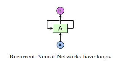
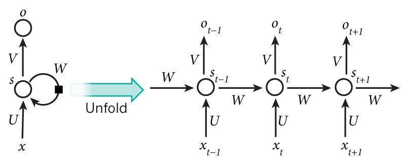
Unfolding the loop( Symbols used) :

• s in the figure represents the state h at any timestep.
  
• (U,V,W) represent the set of weights which we will collectively address as W.
  
• x represents the input at any timestep.
  
• o represents the output at any timestep which we will not talk about here.
  

For a RNN :

The hidden state h_t at time t is a function of the present input x_t and previous state h_t-1. The subscript W in the above recurrence formula refers to the set of weights – the same function f and the parameters W used at every timestep.

At any timestep t, h_t-1 can be viewed as a kind of loose summary of the past sequence of inputs upto time t and thus we can say that the present state of the network is dependant on the entire sequence of inputs upto present time. Depending on training, the network learns how much importance to give to which aspects of the past -some aspects from the past might be more useful to give the desired output at the present time and thus they need to be remembered with more precision than others.

The problem of long term dependencies :

Suppose there is large gap between two related phrases in the text. Theoritically, RNN must not face any difficulty, but RNN's find it difficult to model such long term dependencies in backpropagation. While backpropagating the errors using the chain rule in the training process to update the weights of any neural network, the gradient of the loss function (the error term) gets multiplied by the weigths of the network.

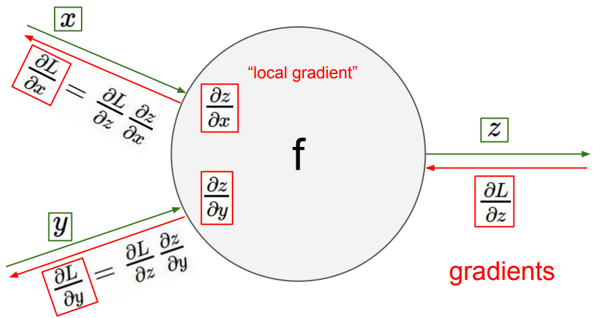
Suppose z = w1x + w2y, than ∂z/∂x = w1 and so ∂L/∂x would also contain the weight w1.

Similarly for vanilla RNN’s :

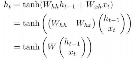
Backpropagation from h_t to h_t-1 involves multiplication by W.

i.e.        ∂L/∂ht-1  = ( ∂L/∂ht )(∂ht/∂ht-1)
                                  would contain the weight W    

The figure explains it better :

Computing gradient of h₀ involves many factors of W multiplied togather.

If W (same for all timesteps)  > 1   =>   Gradient will explode until it reaches h0 
                               < 1   =>   Gradient will vanish until it reaches h0  

So we have these two problems : Exploding Gradients and Vanishing Gradients while modelling long term dependencies with vanilla RNN’s.

Addressing the problem of Exploding gradients : Gradient Clipping

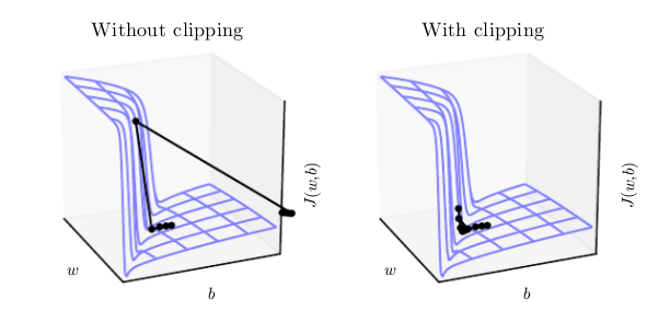
The objective function L(loss function to be minimized ) can be viewed as a landscape with the parameter(w and b in this case) updates via gradient descent being analogous to taking steps in the direction in which the slope is steepest. Traditionally learning rate is there to determine the step size and the gradient determines the direction.

Now, if the magnitude of the parameter gradient is very large (exploding gradient) the parameter update, though being in the right direction would have a very large step size and thus will land us at a region very far away from our current position, which may again not be the minimum of our objective function. Thus we will miss the minimum as shown in 1st figure undoing much of the work that had been done to reach the current position (overshoot).

To prevent this, we can clip the magnitude of the gradients to some threshold before the update.

We can either do element-wise clipping - the parameter gradient in this case is a vector having two components (one w.r.t. b and another w.r.t w), so we can clip both the components individually, or we can clip the norm of the gradient. The latter method guarantees that each step is still in the true gradient direction with only the step size reduced while in element wise clipping, the direction of update is not aligned with the true gradient but is still a descent direction.

Addressing the problem of Vanishing gradients : LSTM's

A nice explanation about LSTM’s can be found here if unfamiliar: Colah's blog

Now in the following section the focus is on how LSTM’s help solve the problem of vanishing gradients.

For LSTM:

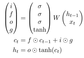
where matrix W = (W_hh W_xh)

• f: Forget gate, how much information to keep from previous timesteps.
• i: Input gate,decides what additional information to add to the cell state c_t-1to get the current state c_t .
• g: Gate gate, multiplied with the input gate.
• o: Output gate, decides how much part of the cell state allowed to flow to the output.

Backpropagation from c_t to c_t-1 involves only elementwise multiplication by f (forget gate), no matrix multiply by W.

i.e.        ∂L/∂ct-1  = ( ∂L/∂ct )(∂ct/∂ct-1) 
                                 will contain f = sigmoid(Whh ht-1 + Wxhxt) instead
                                 of weight W so no repeated multiplication by the
                                 same set of weights W leading to gradient vanishing.

The figure makes it more comprehensible:

LSTM’s can learn long term dependencies by enforcing constant error flow through “constant error carrousels (CEC’s)” via their internal architecture within special units called cells.....three memory cells are shown above. They are designed specifically for this purpose.

The following blog can be referred to learn much of the maths involved :
LSTM backpropagation

P.S. : The content here for Vanishing gradients problem is what I understand.....also I wasn't able to find many sources to learn from for this particular subsection, suggestions and corrections are welcome :)

References :
In addition to the resources mentioned earlier, the following proved to be useful and could be referred further:
1) Deep Learning book by Ian Goodfellow - Chapter 10
2) CS231n Course notes